Problem 1

Given the dynamics and constraints outlined above, the trajectory which maximises the final mass of the rocket (equivalent to minimising the loss in mass) is described as follows:

\[\begin{align*} \max_{t_f, T_c(\bullet)} m(t_f) &= \min_{t_f, T_c(\bullet)} \int_{0}^{t_{f}} ||T_c(t)|| dt \\ \text{subject to } \ddot{r}(t) &= g + \frac{T_c(t)}{m(t)}, \hspace{1cm} \dot{m}(t) = - \alpha ||T_c(t)|| \\ 0 < \rho_{1} &\leq ||T_c(t)|| \leq \rho_{2}, \hspace{0.6cm} r_1(t) \geq 0 \\ ||S_j x(t) - v_j|| &+ c^T_j x(t) + a_j \leq 0, \hspace{0.5cm} j = 1, \ldots, n_s \\ m(0) = m_{wet}&, \hspace{0.8cm} r(0) = r_0, \hspace{0.9cm} \dot{r}(0) = \dot{r}_0 \\ &\hspace{0.15cm} r(t_f) = \dot{r}(t_f) = 0 \end{align*}\]

The thrust magnitude constraint, inequality (3), is a nonconvex constraint on the control input and so we need to deal with it in order to obtain a convex optimisation problem.

We will also add the constraint that \(m(t) > 0\), the paper only adds this in Remark 8, I don’t know why. In Açıkmese et al. (2008) they add the constraint \(m(t_f) \geq 0\) to their problem, in Blackmore, Açikmeşe, and Scharf (2010) they add the constraint \(m(t_f) \geq m_{dry}\) and in Açıkme¸se, Iii, and Blackmore (2013) they add \(m(t_f) \geq m_{dry} > 0\)

Thrust direction can also be constrained at the start and at the end of a manoeuvre as \[\begin{align*} T_c(0) = ||T_c(0)|| \hat{n}_0, \hspace{1.5cm} T_c(t_f) = ||T_c(t_f)|| \hat{n}_f \tag{12} \end{align*}\] where \(\hat{n}_0\) and \(\hat{n}_f\) are unit vectors describing the desired thrust directions.

Problem 2

The modified version of Problem 1 is as follows:

\[\begin{align*} \min_{t_f, T_c(\bullet), \Gamma(\bullet)} \int_{0}^{t_f} \Gamma(t) \,&dt \hspace{1cm} \text{subject to } \dot{m}(t) = - \alpha \Gamma (t) \tag{13} \\ &||T_c(t)|| \leq \Gamma(t) \tag{14} \\ 0 &< \rho_1 \leq \Gamma(t) \leq \rho_2 \tag{15} \\ \ddot{r}(t) &= g + \frac{T_c(t)}{m(t)}, \hspace{1cm} r_1(t) \geq 0 \\ ||S_j x(t) - v_j|| &+ c^T_j x(t) + a_j \leq 0, \hspace{1cm} j = 1, \ldots, n_s \\ m(0) &= m_{wet}, \hspace{0.6cm} r(0) = r_0, \hspace{0.5cm} \dot{r}(0) = \dot{r}_0 \\ &\hspace{0.15cm} r(t_f) = \dot{r}(t_f) = 0 \end{align*}\]

Problem 2 has introduced a slack variable \(\Gamma\) which replaces \(|| T_c ||\) and introduces a new constraint \(\left \lVert T_c(t) \right \rVert \leq \Gamma(t)\). You can see in the figures below, how the control constraint has been mapped to a convex set.

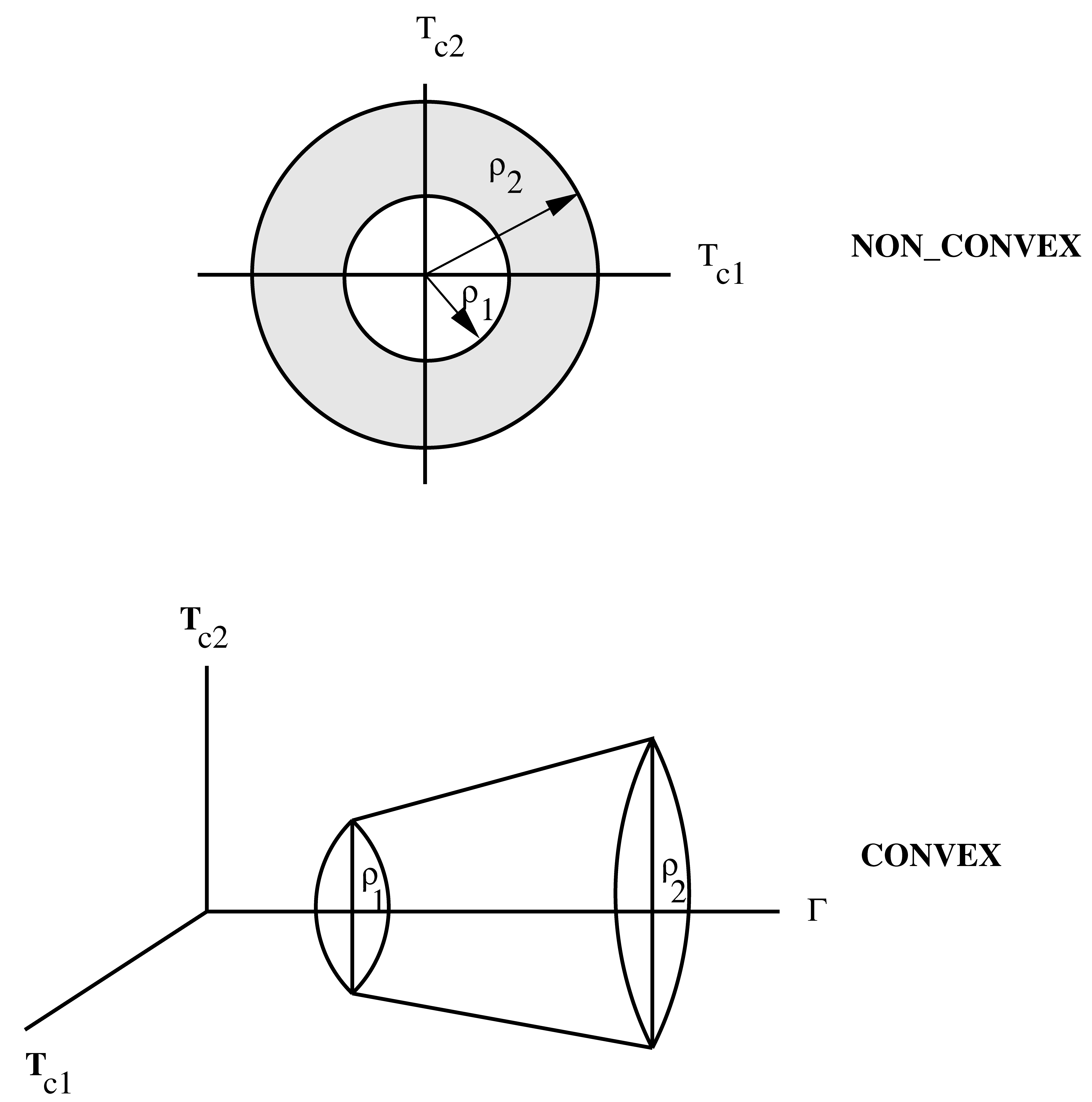
Figure 1: Acikmese and Ploen (2007)

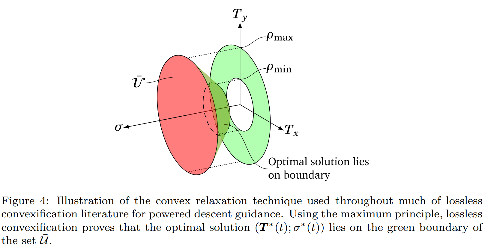
Figure 2: Malyuta et al. (2021)

A solution to Problem 1 is clearly a feasible solution of Problem 2 as we can simply set \(\Gamma(t) = ||T_c(t)||\), however the converse needs to be proved and so below it wil be shown that an optimal solution of Problem 2 is also an optimal solution of Problem 1, which allows us to solve Problem 1 by solving the convex Problem 2.

You might want to check out my notes on Pontryagin’s principle first if you don’t already understand it.

Starting with the first necessary condition (17), we can see that⁴ \[\begin{align*} \frac{\partial H}{\partial y} \left( y^*,\ v^*,\ \lambda_0,\ \lambda \right) &= [ 0,\ \lambda_1,\ \lambda_2^T T^*_c * -\frac{1}{m^2} ]^T \\ \therefore \dot{\lambda}_1 &= 0 \tag{19} \\ \dot{\lambda}_2 &= -\lambda_1 \tag{20} \\ \dot{\lambda}_3 &= \frac{1}{m^2} \lambda_2^T T^{*}_{c} \end{align*}\]

Now onto the transversality condition, let us first construct the set of feasible initial and final conditions \(\left[0,\ y(0),\ t_f,\ y(t_f) \right]\). We know \(y(0)\) is the point \([r_0, \dot{r}_0, m_{wet}]^T\) and \(y(t_f) = [0, 0, 0, 0, 0, 0, m(t_f)]\)⁵, so the the only values in the set that can vary are \(t_f\) and \(m(t_f)\). If a vector is orthogonal to a set at a point, it’s dot product with the tangent vectors to the set at the point will be 0. The tangent vectors to the set are \[\begin{align*} \left. \frac{\partial}{\partial t_f} \right|_{t_f=t_f^*} \left[0, y(0), t_f, y(t_f) \right] = e_9, \hspace{0.5cm} \left. \frac{\partial}{\partial m(t_f)} \right|_{m(t_f)=m(t_f^*)} \left[0, y(0), t_f, y(t_f) \right] = e_{16} \end{align*}\] So \[\begin{align*} [ H(\psi(0)),\ -\lambda(0)^T,\ -H(\psi(t^*_f)),\ \lambda(t_f^*)^T ]^T \cdot e_9 = 0 \end{align*}\] giving \(-H(\psi(t^*_f)) = 0\)⁶ and similarly \(\lambda_3(t^*_f) = 0\).

Now we will show by contradiction that the statement \(\lambda_2(t) = 0 \; \forall \; t \in [0, t_f^*]\) is false. Let’s assume the statement is true, then \(\dot{\lambda}_3 = 0\) and we know \(\lambda_3(t_f^*) = 0\) so \(\lambda_3 = 0\). We also know \(\dot{\lambda}_2 = 0\) if it is always 0 and so \(\lambda_1 = 0\). Since \(H(\psi(t_f^*)) = \lambda_0 \Gamma = 0\), \(\lambda_0 = 0\) which violates the first necessary condition \([\lambda_0,\ \lambda^T]^T \neq 0 \; \forall \; t \in [0,\ t^*_f]\). Therefore the statement is false.

As \(\lambda_1\) is a constant, \(\lambda_2 = -\lambda_1 t + a\) for some constant a. As we know \(\lambda_2\) is not identically zero then \(\lambda_2\) can be zero, at most, at one point on \([0, t_f^*]\).

We can express the Hamiltonian as \[\begin{align*} H(x, m, T_c, \Gamma, \lambda_0, \lambda) = R_1(t) \Gamma + R_2(t)^T T_c + R_0(t) \tag{21} \end{align*}\] where \[\begin{align*} R_0(t) = \lambda_1(t)^T x_2(t) + \lambda_2(t)^T &g, \hspace{1cm} R_1(t) = \lambda_0 -\alpha \lambda_3(t) \\ R_2(t) &= \frac{\lambda_2(t)}{m(t)} \end{align*}\]

To maximise the Hamiltonian per the pointwise maximum principle (18) we want to maximise \(R_2(t)^T T_c(t) = ||R_2(t)|| \ ||T_c(t)|| \cos \theta(t)\), we want to maximise \(||T_c(t)|| \cos \theta(t)\) unless \(||R_2(t)|| = 0\). \(||R_2(t)|| = 0\) iff \(\lambda_2(t) = 0\) as \(m^*(t) \neq 0\) and because \(\lambda_2(t) \neq 0\) a.e. on \(t \in [0, t_f^*]\) then we want to maximise \(||T_c(t)|| \cos \theta\) a.e. on \(t \in [0, t_f^*]\). So we want to maximise \(||T_c(t)||\) as long as \(\cos \theta(t) > 0\). As we can choose \(\theta(t)\) without constraint for \(t \in (0, t^*_f)\)⁷, we choose \(\cos \theta(t) = 1\) for all \(t \in (0, t^*_f)\). The maximum of \(||T_c(t)||\) is \(\Gamma(t)\) per \(\Psi\) so \[\begin{align*} ||T^*_c(t)|| &= \Gamma^*(t) \text{ a.e. on } [0, t^*_f] \tag{22}\\ T^*_c &= \frac{R_2}{||R_2||} \Gamma^* \text{ a.e. on } t \in [0, t_f^*] \ (\text{as } ||R_2|| \neq 0 \text{ a.e. on } [0, t_f^*]), \\ \rho_1 &\leq ||T^*_c(t)|| \leq \rho_2 \text{ a.e. on } t \in [0, t_f^*] \end{align*}\]

Therefore an optimal solution of Problem 2 satisfies all the constraints of Problem 1 and the objective function is the same so it also defines an optimal solution for Problem 1.

Now we will show that \(||T_c^*(t)|| = \rho_1\) or \(||T_c^*(t)|| = \rho_2\) for any \(t \in [0, t_f^*]\) by using the pointwise maximum principle. We can now see that⁸ \[\begin{align*} H(x, m, T_c, \Gamma, \lambda_0, \lambda) &= H(\psi(t)) = R_{12}(t) \Gamma + R_0(t), \\ \text{ where } R_{12}(t) &= R_1(t) + ||R_2(t)|| \end{align*}\]

The pointwise maximum principle implies that \[\begin{align*} \Gamma^*(t) = \begin{cases} \rho_1, & \text{if } R_{12}(t) < 0 \\ \rho_2, & \text{if } R_{12}(t) > 0 \end{cases} \end{align*}\] We can ignore the \(R_{12}(t) = 0\) case as we can show that \(R_{12}(t) \neq 0\) a.e. on \(t \in [0, t_f^*]\).

As \(R_1(t) = \lambda_0 - \alpha \lambda_3(t)\) we note that \[\begin{align*} \dot{R}_1(t) &= -\alpha \frac{1}{m^2}\lambda_2^T T^*_c \\ &= - \frac{\alpha}{m} R_2^T T^*_c \\ &= - \frac{\alpha}{m} R_2^T \frac{R_2}{||R_2||} \Gamma^* \\ &= - \frac{\alpha}{m} ||R_2|| \Gamma^* \end{align*}\]

Also by noting that \(||R_2|| = \frac{||\lambda_2||}{m}\) (as \(m > 0\)) note that \[\begin{align*} \frac{d ||R_2||}{d t} &= \frac{1}{m} \frac{d ||\lambda_2||}{d t} - \frac{\dot{m}}{m^2} ||\lambda_2|| \\ &= \frac{1}{m} \frac{d ||\lambda_2||}{d t} + \frac{\alpha \Gamma^*}{m^2} ||\lambda_2|| \\ &= \frac{1}{m} \frac{d ||\lambda_2||}{d t} + \frac{\alpha}{m} ||R_2|| \Gamma^* \end{align*}\]

So \[\begin{align*} m \dot{R}_{12} &= m\dot{R}_1 + m \dot{||R_2||} \\ &= - \alpha ||R_2|| \Gamma^* + \frac{d ||\lambda_2||}{d t} + \alpha ||R_2|| \Gamma^* \\ &= \frac{d ||\lambda_2||}{d t} \\ &= -\frac{\lambda_2^T}{||\lambda_2||} \lambda_1 \\ &= -\frac{1}{||\lambda_2||} (-\lambda_1 t + a)^T \lambda_1 \\ &= \frac{1}{||\lambda_2||} (\lambda_1^T \lambda_1 t - a^T \lambda_1) \\ &= \frac{1}{||\lambda_2||} (||\lambda_1||^2 t - \lambda_1^T a) \end{align*}\]⁹ where \(\lambda_1\) and \(a\) are constant vectors and they cannot both be zeros as that would imply that \(\lambda_2\) is identically 0 and we know this to be false.

If \(\lambda_1 \neq 0\) then \(m \dot{R}_{12}\) is not identically 0 and as \(m \neq 0\) we know \(\dot{R}_{12}\) is not identically 0. When \(\lambda_1 \neq 0\), we can see that \(\frac{d}{dt} m \dot{R}_{12} = \frac{||\lambda_1||^2}{||\lambda_2||} > 0\), so \(m\dot{R}_{12}\) can only be zero at one point and the sign can only change from negative to positive. As \(m > 0\) the sign of \(\dot{R}_{12}\) is the same as \(m\dot{R}_{12}\), there can only be two points at maximum where \(R_{12} = 0\) so \(R_{12} \neq 0\) a.e. on [0, t_f] when \(\lambda_1 \neq 0\).

Note that \(\dot{R}_{12} = 0\) on some interval \([t_a, t_b]\) which is a subset (don’t think it has to be strict) of \([0, t_f]\) only if \(\lambda_1 = 0\). If \(\lambda_1 = 0\) then \(\dot{R}_{12} = 0 \; \forall \; t \in [0, t_f]\), so to show \(R_{12} \neq 0\) we still need to show that \(R_{12}\) is not identically 0 when \(\lambda_1 = 0\). To do this, suppose that \(R_{12}\) is identically 0 when \(\lambda_1 = 0\). This implies \(\lambda_2\) is constant in time and \[\begin{align*} H(\psi(t_f^*)) = R_0(t) + R_{12}(t)\Gamma^*(t) = R_0(t) = 0 \\ R_0(t) = \lambda_1(t)^T x_2(t) + \lambda_2(t)^T g = g^T \lambda_2(t) = 0 \end{align*}\]

Since \(T_c^* = \frac{R_2}{||R_2||}\Gamma^* = \frac{\lambda_2}{||\lambda_2||} \Gamma^*\) then \(g^T T_c^* = g^T \lambda_2 \frac{R_2}{||\lambda_2||} = 0\).

Recall \(\ddot{r}(t) = g + \frac{T_c(t)}{m(t)}\), where \(g\) is a constant and \(\frac{T_c^*(t)}{m(t)} = \frac{\Gamma^*(t)}{m(t)} \hat{n}\) is always pointing in the direction of \(\hat{n}\), letting \(\hat{n} = \frac{\lambda_2}{||\lambda_2||}\) which is a constant. The \(\frac{T_c^*(t)}{m(t)}\) component will therefore only affect velocity in the \(\hat{n}\) direction. Therefore \(\dot{r}(t) = g t + \beta(t) \hat{n} + \dot{r}_0\)¹⁰ and so \(\dot{r}(t_f) = g t_f + \beta_2 \hat{n} + \dot{r}_0 = 0\). Integrating \(\dot{r}(t)\) we get \(r(t) = r_0 + \dot{r}_0 t + g \frac{t^2}{2} + B(t) \hat{n}\).¹¹ So \(r(t_f) = r_0 + \dot{r}_0 t_f + g \frac{t_f^2}{2} + \beta_1 \hat{n} = 0\).

Recall \(g^T T_c^* = 0\) and \(T_c^* = \Gamma^* \hat{n}\) so \(g^T \hat{n} = 0\). Then \[\begin{align*} -\frac{g^T}{||g||} \dot{r}(t_f) &= -||g|| t_f - \frac{g^T}{||g||} \beta_2 \hat{n} - \frac{g}{||g||} \dot{r}_0 \\ &= -||g|| t_f + \dot{r}_{0_1} \\ &= 0 , \end{align*}\] remember \(\dot{r}_{0_1} = -\frac{g^T}{||g||} \dot{r}_0\). Also \[\begin{align*} -\frac{g^T}{||g||} r(t_f) &= r_{0_1} + \dot{r}_{0_1} t_f - ||g|| \frac{t_f^2}{2} \\ &= 0 , \end{align*}\] remember \(r_{0_1} = -\frac{g^T}{||g||} r_0\).

\[\begin{align*} \dot{r}_{0_1} &= ||g|| t_f \geq 0\\ r_{0_1} &= ||g|| \frac{t_f^2}{2} - \dot{r}_{0_1} t_f \\ &= ||g|| \frac{t_f^2}{2} - ||g|| t_f \\ &= -||g|| \frac{t_f^2}{2} \\ &= -\frac{\dot{r}_{0_1}^2}{2||g||} \leq 0 \end{align*}\] Recall we assumed \(r_{0_1} > 0\) in (6), which leads to a contradiction. Therefore, \(R_{12}(t) \neq 0 \; \forall \; t \in [0, t_f]\) when \(\lambda_1 = 0\) and so \(R_{12}(t) \neq 0\) a.e. on \([0, t_f^*]\).

The proof of Lemma 1 is thus complete. Lemma 1 implies that main nonconvex constraint on the thrust magnitude (3) in Problem 1 is convexified by replacing it with (14) and (15) in Problem 2 via the introduction of a slack variable \(\Gamma\). Furthermore, Lemma 1 states that if there exists and optimal solution for Problem 2, then there also exist one for Problem 1 and it can be obtained directly from the optimal solution of Problem 2.

To add the start/end thrust direction constraints (12) to Problem 2 we use (22) to get the constraints \[\begin{align*} T_c(0) = \Gamma(0) \hat{n}_0, \hspace{1cm} T_c(t_f) = \Gamma(t_f) \hat{n}_f \tag{23} \end{align*}\]

Existence of an Optimal solution

Now before we try to solve Problem 2 to obtain an optimal solution, we have to first make sure that an optimal solution exists.

Brief Interlude - Boundary Value Problem

When using the Pontryagin’s principle you may solve a two-point boundary-value problem to obtain the optimal control. I lay it out below.

We have \(x = [r, \dot{r}, m]\) where \(r \in \mathbb{R}^3\) and \(m \in \mathbb{R}\). We also have \(\lambda = [\lambda_1, \lambda_2, \lambda_3]\) where \(\lambda_1, \lambda_2 \in \mathbb{R}^3\) and \(\lambda_3 \in \mathbb{R}\). \(g\) is the gravity vector and \(\alpha\) is a given scalar coefficient. \[\begin{align*} \dot{x} &= \begin{bmatrix} \dot{r} \\ g + \frac{\lambda_2}{||\lambda_2||} \Gamma \\ - \alpha \Gamma \end{bmatrix} \\ \dot{\lambda} &= - \begin{bmatrix} \boldsymbol 0 \\ \lambda_1 \\ ||\lambda_2|| \Gamma / m^2 \end{bmatrix} \end{align*}\] where \[\begin{align*} R_{12}(t) = \lambda_0 - \alpha \lambda_3 + \frac{||\lambda_2||}{m} \\ \Gamma(t) = \begin{cases} \rho_1, & \text{if } R_{12}(t) < 0 \\ \rho_2, & \text{if } R_{12}(t) > 0 \end{cases} \end{align*}\] \(x(0)\) is given and \(r(t_f), \dot{r}(t_f) = \boldsymbol 0\), where \(t_f\) is the final time, it is free and \(t_f > 0\). Also \(\lambda_3(t_f) = 0\), \(H(t_f) = \lambda_0 \Gamma + \lambda^T \dot{x} = 0\), \(\lambda_0 = 0\) or \(-1\) and \(\lambda \neq 0\) for all \(t \in [0, t_f]\).

Unfortunately, I have found that solving this problem seems difficult. I tried using the bvp4c solver in matlab which complained about a singular jacobian matrix even if I gave the analytic jacobian. I also used a few different solvers in julia which would give a result that didn’t satisfy the boundary constraints or would complain about dt <= dtmin. I’ve given up on trying to numerically solve it, I just thought it would be much simpler than what the paper did but I have no experience with numerical methods in general. I figure I need to give it a better initial guess for the adjoint equations or the bang bang control is giving problems.

Additionally, I have found the following quote ‘solving the resulted two-point boundary value problem is a difficult task, and good initial guesses of the adjoint variables can be difficult to find or compute’ Lysandrou (2018), which backs up my experience. Also, ‘issues that hinder onboard implementation include poor convergence stemming from a sensitivity to the initial guess, and long computation time.’ Malyuta et al. (2021)

Change of Variables

In this section a change of variables is introduced to remove the nonlinear state dynamics due to \(\frac{T_c}{m}\) Blackmore, Açikmeşe, and Scharf (2010) Açıkme¸se, Iii, and Blackmore (2013).

I don’t think I am going to make notes on the rest of this paper or the following papers as I was able to skim it well enough to implement the results for a rocket with solid motors.

Note Nonlinear Optimal Control Theory by Leonard David Berkovitz, Negash G. Medhin is the sequel to citation 23 in Acikmese and Ploen (2007)